1) What process does expressing color numerically actually involve?
CIE 1931 Colorimetry provides theoretical and experimental foundations to explain how the human visual system perceives various spectral distributions as colors. Imagining cases like tree leaves and green cars that appear the same color but have completely different reflection spectra shows that identical color perception can occur under different physical conditions. This phenomenon where different spectral distributions induce identical color stimuli is called metamerism, a core concept of color reproduction.
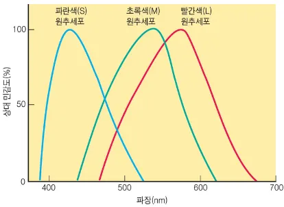
Fig 1. Wavelength-dependent relative sensitivity distribution of human cone cells (S/M/L).
Metamerism means the original spectrum isn’t necessarily required to reproduce a color. In other words, if a combination can induce identical cone cell responses in humans, it’s perceived as the same color even without the original light source. For example, LCD displays can implement conditions the human visual system perceives as yellow by properly combining red and green light sources, even without generating spectral yellow.
CIE 1931 XYZ color space mathematically established and modeled this color matching principle. This is the reference color space proposed by the International Commission on Illumination (CIE) to reproduce identical colors regardless of lighting conditions or display devices, and is the first standard mathematically defining color. CIE XYZ is based on Trichromatic Theory, expressing colors through three imaginary primary stimuli (X, Y, Z). This model becomes the basis for defining various color spaces like RGB, LAB, HSV, and is used as a reference coordinate system across colorimetry, printing, and display industries.
2) 1924 Luminous Efficiency Function, V(λ)
The 1924 CIE luminous efficiency function V(λ), which can be considered a predecessor of this model, defined standards for human brightness perception before color stimuli. V(λ) indicates how sensitively the human eye responds to each wavelength in the visible light range, showing maximum response around 555nm greenish light. This function shows that two wavelengths with identical physical brightness (radiant flux) can actually appear different. For instance, if blue and green lights appear equally bright, physically the blue light has higher radiance.
This numerically expresses that the human visual system doesn’t respond equally across wavelengths. For example, if green and blue lights appear equally ‘bright,’ it means the blue light actually has higher radiance. V(λ) became an important standard for understanding the gap between visual uniformity and physical uniformity.
However, the 1924 version of V(λ) was later found to underestimate human sensitivity response in the blue region of the spectrum. This has been improved through subsequent modeling and corrections, and the CIE 1931 colorimetry model established itself as the first comprehensive system quantifying overall color perception including such luminous response.
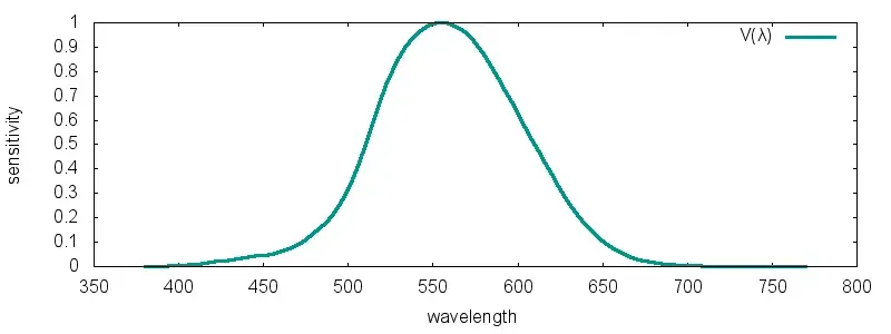
Fig. 2. CIE 1924 luminous efficiency function V(λ) and wavelength-dependent brightness perception characteristics.
3) Properly Reading the “Color Gamut Graph”: CIE 1931 xy
Human vision receives light spectrum $I(\lambda)$ composed of various wavelengths and perceives it as color. CIE 1931 standard observer functions emerged to mathematically formalize this process. The three color matching functions (CMFs) used at this time are $\bar{x}(\lambda),\ \bar{y}(\lambda),\ \bar{z}(\lambda)$ respectively—functions constructed to express all colors humans can perceive with three imaginary primaries.
These functions were derived through ‘Wright-Guild Color Matching Experiments’ with numerous subjects under 2-degree viewing conditions. The experimental method set reference wavelengths at 10nm intervals and found combinations that appeared identical to reference colors by adjusting the intensity of three primary light sources—red (700nm), green (546.1nm), blue (435.8nm). Subjects had to create combinations that felt identical to reference colors by mixing these three monochromatic lights, and numericalizing those combinations became tristimulus values.
However, experimental results showed that for some wavelengths, reference colors couldn’t be implemented with only positive combinations of RGB primaries, leading to the introduction of negative values. For example, bright green near 520nm could only be expressed using red with negative values, and the concept of negative light was used to quantitatively explain areas unreproducible with RGB. These results were solved by actually adding negative light sources to the other side rather than the reference color to accurately match colors.
The $\bar{x}(\lambda),\ \bar{y}(\lambda),\ \bar{z}(\lambda)$ functions thus generated are color matching functions based on imaginary primaries that mathematically reconstructed experimental results to explain human color matching behavior.
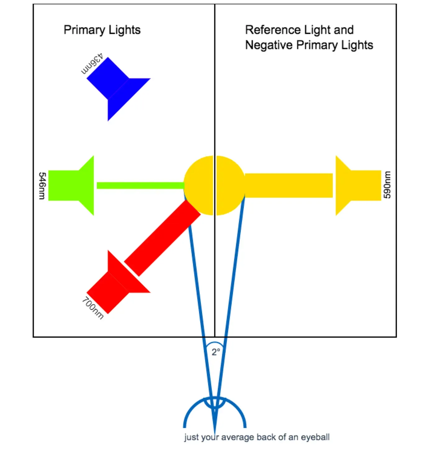
Fig. 3. Conceptual structure of Wright–Guild color matching experiment.
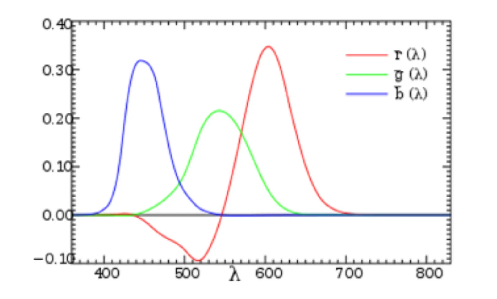
Fig. 4. Negative stimulus value phenomenon appearing in RGB color matching functions.
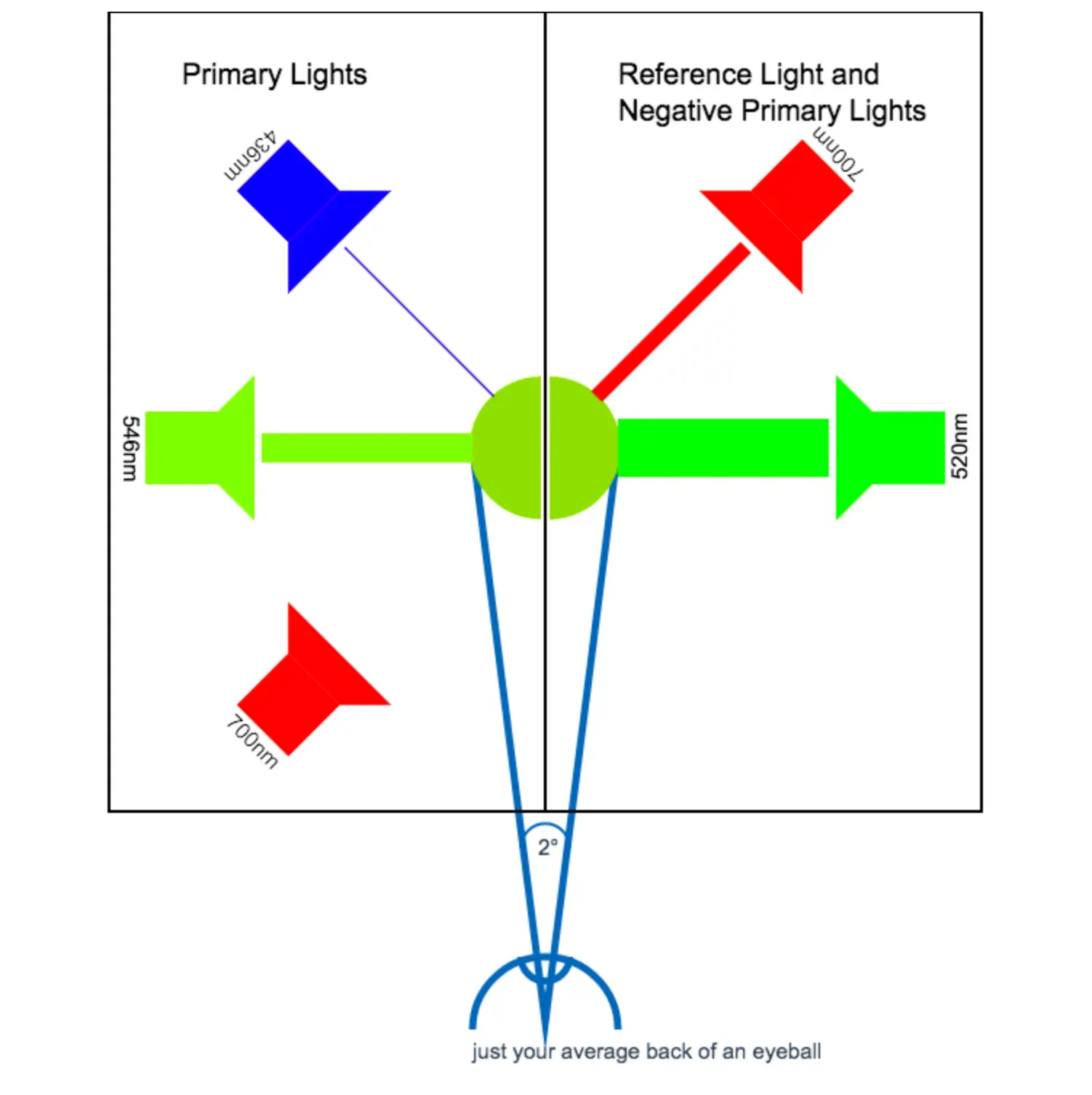
Fig. 6. Experimental derivation process of CIE 1931 color matching functions and standard observer model.
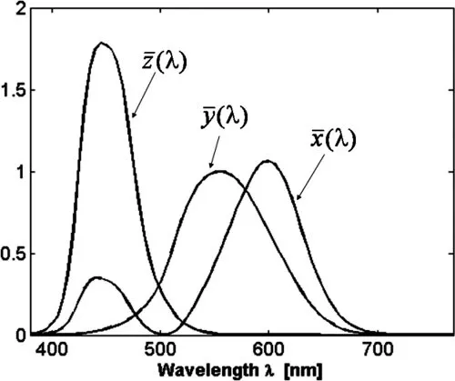
Fig. 5. CIE 1931 color matching functions x̄(λ), ȳ(λ), z̄(λ).
4) Mathematical and Visual Process Defining the Chromaticity Diagram (CIE 1931 Chromaticity Diagram)
Tristimulus values (XYZ) are very useful systems for numerically defining color, but because they’re interpreted in 3-dimensional space composed of three axes (X, Y, Z), intuitive visual understanding is difficult. Accordingly, CIE additionally defined a 2-dimensional color space in 1931 based on XYZ values but with luminance information removed. This is what’s commonly called the CIE 1931 chromaticity diagram.
To mathematically express human color perception, CIE defined three independent reference functions $\bar{x}(\lambda),\ \bar{y}(\lambda),\ \bar{z}(\lambda)$. These are weighting functions indicating how humans respond to each wavelength λ, serving as a kind of basis. Taking the inner product of spectral distribution $I(λ)$ with these three functions yields tristimulus values X, Y, Z. These values are conceptually defined as follows:
$$ X=k⋅\bar{x}(λ) \ Y=k⋅\bar{y}(λ) \ Z=k⋅\bar{z}(λ) $$
Or expressed as inner products for general spectrum $I(λ)$ as follows. Here X, Y, Z are absolute color stimuli, including not just color information but also brightness information.
$$ X=⟨I(λ),\bar{x}(λ)⟩ \ Y=⟨I(λ),\bar{y}(λ)⟩\ Z=⟨I(λ),\bar{z}(λ)⟩ \ $$
Since the above inner product operations are defined for continuous spectra, they’re actually calculated in integral form. Each stimulus value is given by the following equations:
$$ X=k∫I(λ)\bar x(λ)dλ \ Y=k∫I(λ)\bar y(λ)dλ \ Z=k∫I(λ)\bar z(λ)dλ $$
Here $k$ is a scaling constant, generally adjusted so Y becomes the reference luminance. Through this calculation we can obtain corresponding tristimulus values (X, Y, Z) for arbitrary spectrum $I(λ)$.
The X, Y, Z values thus obtained are considered absolute color stimulus values including brightness information. However, when constructing chromaticity diagrams, only pure color attributes with brightness information removed are needed, so XYZ values are normalized and converted to chromaticity coordinates x, y, z. Each value is defined as follows:
$$ x=\frac{X}{X+Y+Z},\ y=\frac{Y}{X+Y+Z} $$
Here $z = \frac{Z}{X + Y + Z}$ is also defined, but since the relationship x+y+z=1 always holds, entire information can be expressed with only x,y.
Repeating the above normalization process for single wavelength λ from 380nm to 700nm generates (x, y) coordinates for each wavelength. Connecting these coordinates forms an outer boundary line on the chromaticity diagram, called the spectral locus. This boundary line is the chromaticity corresponding to monochromatic light, and the straight line connecting below the curve is called the line of purples. The following figure shows an example.
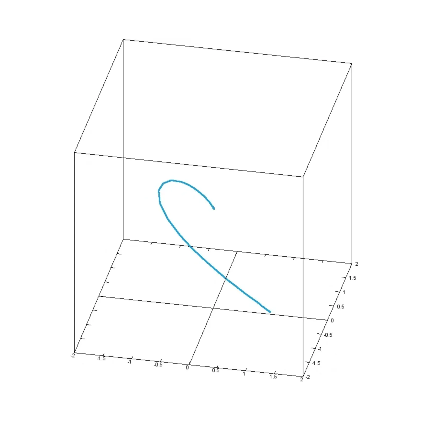
Fig. 8. Trajectory formed by monochromatic spectrum in XYZ space.
Chromaticity diagram (x, y) coordinates normalizing tristimulus values can be interpreted as unit vectors leaving only vector direction. Since the sum of three values is fixed at 1, knowing the first two values automatically determines the remaining one. This also relates to the concept of dimensionality reduction.
The same principle applies in RGB space. Removing intensity (brightness) information enables projection from 3-dimensional to 2-dimensional rg plane, and for purposes of analyzing only chromaticity, such 2-dimensional projection makes visualization much simpler.
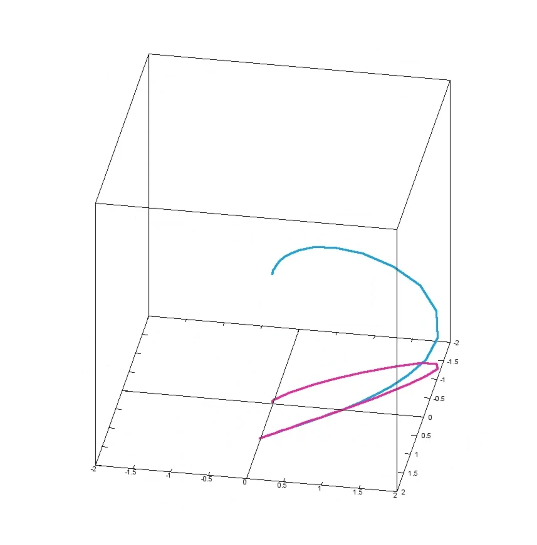
Fig. 7. 3D → 2D projection (rg plane projection) example
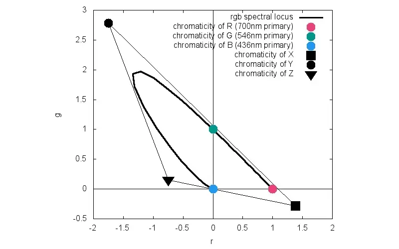
Fig. 9. rg chromaticity plane and RGB gamut representation.
- Each point on the outer curve corresponds to monochromatic light (spectral colors).
- Points inside the curve represent non-spectral colors mixed from two or more wavelengths.
- Chromaticity outside the curve is an area unrealizable with monochromatic or general mixed light.
- RGB primaries correspond to monochromatic light so are located on the curve boundary.
- Colors inside the triangle formed by three RGB color points are areas realizable with those RGB light sources, and colors outside the triangle need more light sources for expression.
Display devices’ color reproduction capability is limited by the physically realizable color gamut. Each display has chromaticity coordinates of its own R, G, B light sources, and the triangular area inside with these three points as vertices determines the chromaticity range expressible by that device. Chromaticity inside this triangle is color reproducible by that device, and outside is considered unreproducible color. The larger the triangle, the wider that device’s color reproduction range.
Most color correction or color temperature adjustment is performed centered on a specific reference point within such color space, namely the white point (e.g., D65). This reference point is located on the color temperature curve, serving as the standard for adjusting color balance in displays.

Fig. 10. Gamut comparison on CIE 1931 chromaticity diagram: sRGB, Adobe RGB, DCI-P3.

Fig. 11. Display device RGB primary color coordinates and gamut triangle representation.
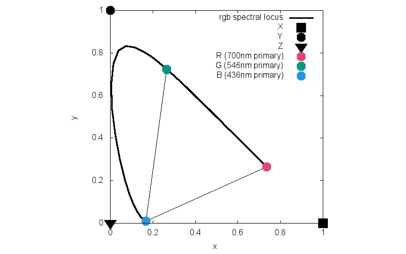
Fig. 12. Color space redefinition process converting RGB chromaticity coordinates (r, g) to XYZ chromaticity coordinates (x, y).
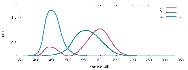
Fig. 13. Construction principle of XYZ color space using Imaginary Primaries.
When mathematically defining color through Color Matching Functions (CMF), if primaries are selected based only on existing colors, RGB tristimulus values experience the problem of negative values occurring at some wavelengths. This means ’negative amounts of color’ must be added to make specific colors, which is physically unrealizable or difficult to interpret.
To solve this problem, CIE introduced imaginary primaries. These imaginary colors are located outside the actual color range, but thanks to this, they can generate positive tristimulus values (XYZ) for all visible light wavelengths. In other words, they enable expressing all spectrum colors visible to the human eye as positive linear combinations.
Such characteristics are impossible in RGB-based color coordinate systems. On the previously examined chromaticity diagram, to construct a triangle containing all actual colors, the triangle’s vertices must be outside the actual color range. XYZ color space is a model constructed to satisfy this condition.
CIE uses the following transformation matrix to convert RGB tristimulus values to XYZ tristimulus values. (This transformation matrix is an example of CIE RGB-based XYZ transformation; actual sRGB, Adobe RGB, etc., use different transformation matrices.)
This transformation matrix has two purposes:
- Adjusting so stimulus values at all wavelengths become positive.
- Correcting so the Y component corresponds with V(λ) function, the human brightness perception curve.
In XYZ color space obtained through this transformation, RGB CMFs all appear as positive values, and explanation without negative stimulus values is possible when expressing colors. This is a very important characteristic in actual display device color management systems. Particularly, Y stimulus value is used as a brightness representative, utilized as a reference value in luminance-based operations or HDR tone mapping.
Visualization of Chromaticity Diagram and Visible Color Range
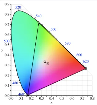
Fig. 14. CIE 1931 chromaticity diagram (xy) and visualization of visible color range.
The CIE 1931 chromaticity diagram (xy) is a reference diagram projecting the chromaticity distribution of visible light spectrum in 2-dimensions based on standard observer standards modeling average human visual system response (measured under 2° conditions). The edge of this diagram, the curve forming a horseshoe shape, corresponds to pure monochromatic light (spectral colors) according to wavelength λ (400–700nm), and this curve represents colors of maximum saturation possible in visible light.
The triangular area existing inside represents the range of colors a specific display device can express, namely the color gamut. Each vertex of this triangle is displayed as the color coordinates (xR, yR), (xG, yG), (xB, yB) of that device’s R, G, B primary colors, and only colors inside the area formed by connecting these can be generated on that device. Other colors are in an out of gamut state, meaning colors technically unreproducible. Additionally, the device’s white point must exist inside this triangle to express actual white, which doesn’t need to exactly match the theoretical center E (Equal Energy White Point), but generally exists at a different location.
CIE 1976 (u′, v′) Uniform Chromaticity Diagram and Improvement of Color Perception
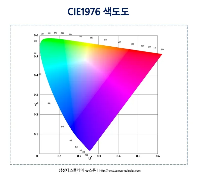
Fig. 15. CIE 1976 (u′, v′) uniform chromaticity diagram and perceptual uniformity improvement effect.
While the existing CIE 1931 chromaticity diagram contributed to effectively visualizing color coordinate space, limitations were also clear. Particularly, the green region was excessively expanded, and the problem existed where identical physical color differences appeared as distance distortions on the chromaticity diagram. In other words, mismatches occurred between color differences humans perceive and distances in the xy chromaticity diagram. This problem clearly revealed itself through size differences of equal-color regions (MacAdam ellipse) between colors—actually near green, one ellipse can be over 10 times larger than blue.
To improve this, CIE introduced the CIE 1976 (u′, v′) Uniform Chromaticity Scale Diagram in 1976. This new chromaticity diagram was mathematically reconstructed to correspond more uniformly to human visual sensitivity, designed so movement of equal distance in each direction feels like equal perceptual difference. As a result, red and blue regions were visually expanded, and overall perceptual uniformity between colors improved. This came to provide much more meaningful standards in color difference calculations or design work based on color perception.
Color Range and Reproduction Limits in the Real World
Most color spaces used in reality (sRGB, Adobe RGB, etc.) don’t completely include the entire horseshoe area on the CIE 1931 chromaticity diagram. This means only part of the total color range humans can perceive is expressible, reflecting physical limits of expressible gamut.
For example, if a digital camera operates based on sRGB color space, if the subject has colors corresponding to outside sRGB’s triangle, that color isn’t accurately reproduced. Instead, it’s expressed replaced by the closest substitutable color within the gamut. This process is called gamut clipping, and similarly occurs in output devices (monitors, printers).
Such limitations are determined by display device primary color coordinates, physical lighting characteristics, sensor sensitivity, etc. Therefore each device has different color expression capability, and is also why color consistency doesn’t happen perfectly between devices even for identical images.
For more details, please refer to Part 1 of this series.
Reference